This article summarizes the stability of systems represented by state equations. Videos related to stability are placed at the bottom.
Poles of the Controlled System and Stability
Here, I will explain the stability of control systems. First, let's assume the following system is given.
\begin{equation} \dot x(t) = Ax(t) + Bu(t) \\ y(t) = Cx(t) \end{equation}
The characteristics of the various parameters are summarized as Basics of State Equations.
At this point, whether the given system is stable or not can be determined by examining the characteristics of Image may be NSFW.
Clik here to view. , particularly characterized by the eigenvalues of matrix Image may be NSFW.
Clik here to view. .
.
Matrix Image may be NSFW.
Clik here to view. is a square matrix, and its eigenvalues can be found by solving the following equation.
\begin{equation} det ( A-\lambda I) = 0\end{equation}
Here, Image may be NSFW.
Clik here to view. is the identity matrix. If Image may be NSFW.
Clik here to view. is an Image may be NSFW.
Clik here to view. matrix, there are Image may be NSFW.
Clik here to view. eigenvalues.
By checking these eigenvalues, if the real parts of all eigenvalues are negative, the system is asymptotically stable.
On the other hand, if the real part of any eigenvalue is positive or zero, the system is unstable or marginally stable.
Here, we will check the stability for both the case where the system order Image may be NSFW.
Clik here to view. and the case where the order Image may be NSFW.
Clik here to view. .
.
When the Order of the Controlled System is 1
Here, we consider a scalar system with one state. Image may be NSFW.
Clik here to view. is a scalar value, not a matrix. When Image may be NSFW.
Clik here to view. , the state equation can be written as follows.
\begin{equation} \dot x(t) = -x(t) + u(t)\end{equation}
The solution of this state equation is
Image may be NSFW.
Clik here to view.
and if Image may be NSFW.
Clik here to view. , Image may be NSFW.
Clik here to view. asymptotically approaches zero over time, regardless of the initial state Image may be NSFW.
Clik here to view. . On the other hand, if Image may be NSFW.
Clik here to view. ,
,
Image may be NSFW.
Clik here to view.
and it diverges. Suppose Image may be NSFW.
Clik here to view. , then the state equation is
\begin{equation} \dot x(t) = u(t) \end{equation}
This means that the integral of the input Image may be NSFW.
Clik here to view. becomes the state Image may be NSFW.
Clik here to view. . For example, if Image may be NSFW.
Clik here to view. is a step signal, the state Image may be NSFW.
Clik here to view. diverges.
When the order of the controlled system is 3
Consider the case where the following matrix Image may be NSFW.
Clik here to view. is given.
\begin{equation} A = \begin{bmatrix} -1 & 0 & 0\\0 &-2&0\\0&0&-3\end{bmatrix}\end{equation}
In this case, the eigenvalues are Image may be NSFW.
Clik here to view. , and since the real parts of all eigenvalues are negative, it is asymptotically stable. When analyzing a control system, eigenvalues are plotted on the complex plane. When plotting the eigenvalues on the complex plane for this example, it looks like the following diagram.
Image may be NSFW.
Clik here to view.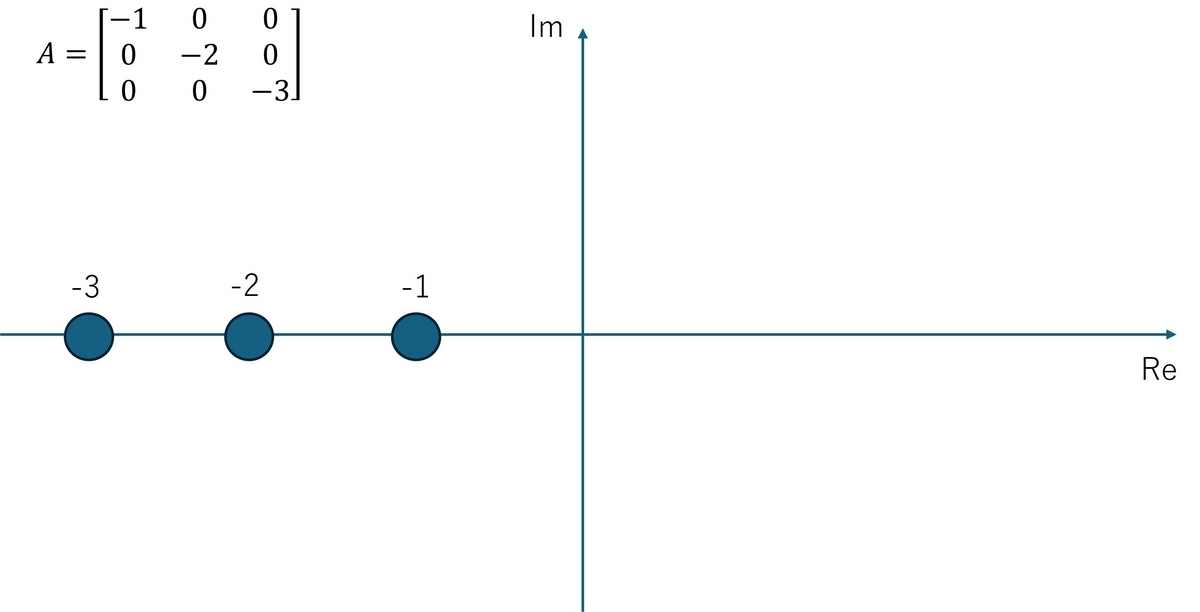
Eigenvalues of the Matrix 01
An example of the response waveform in this case is shown.
Image may be NSFW.
Clik here to view.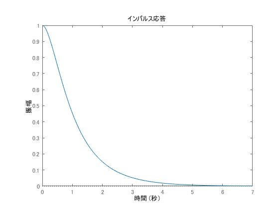
Next, consider the case where Image may be NSFW.
Clik here to view. is given by the following equation.
\begin{equation} A = \begin{bmatrix} -1 & 0 & 0\\0 &-2&-1\\0&1&-2\end{bmatrix}\end{equation}
In this case, the eigenvalues are Image may be NSFW.
Clik here to view., and since the real parts of all eigenvalues are negative, it is asymptotically stable, similar to the previous case. When plotting the eigenvalues on the complex plane for this example, it looks like the following diagram.
Image may be NSFW.
Clik here to view.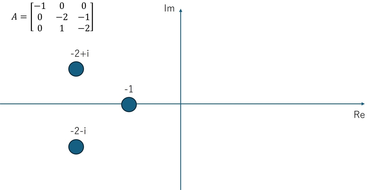
Eigenvalues of the Matrix 02
An example of the response waveform in this case is shown.
Image may be NSFW.
Clik here to view.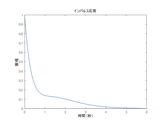
Finally, consider the case where Image may be NSFW.
Clik here to view. is given by the following equation.
\begin{equation} A = \begin{bmatrix} -1 & 0 & 0\\0 &1&-1\\0&1&1\end{bmatrix}\end{equation}
In this case, the eigenvalues are Image may be NSFW.
Clik here to view., and since it includes an eigenvalue with a positive real part, it is unstable. When plotting the eigenvalues on the complex plane for this example, it looks like the following diagram.
Image may be NSFW.
Clik here to view.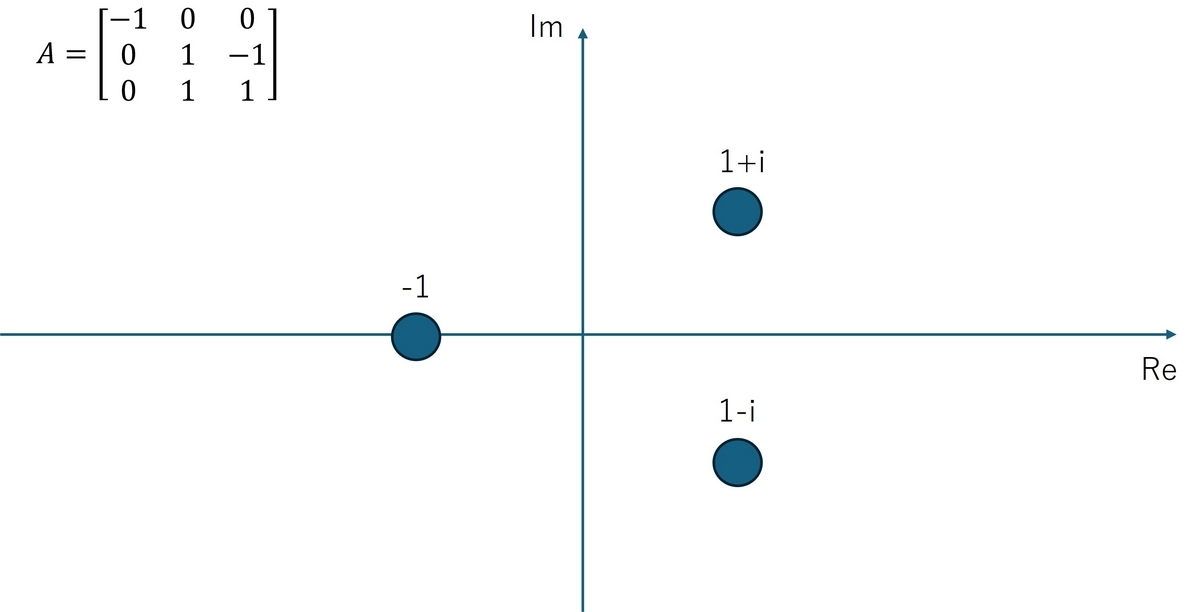
Eigenvalues of the Matrix 03
An example of the response waveform in this case is shown.
Image may be NSFW.
Clik here to view.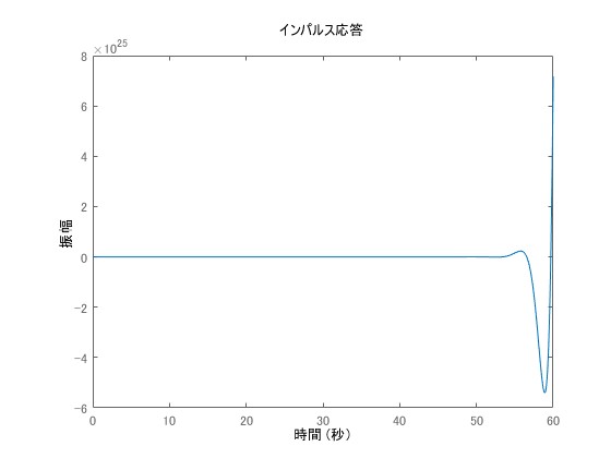
This concludes the explanation of eigenvalues of matrices and stability. Design is performed while observing not only stability but also the characteristics of the response. Pole placement is explained in the following article.
Lyapunov's Stability Criterion
Now, I will explain Lyapunov's stability criterion. Lyapunov's stability criterion is a powerful method for determining the stability of autonomous systems without solving for the solution.
It is a quite powerful tool, capable of handling nonlinear systems. The basic idea is as follows.
First, consider a scalar-valued function Image may be NSFW.
Clik here to view.. This is a positive definite function that is always positive for any Image may be NSFW.
Clik here to view.. For example,
\begin{equation} V(x)=x^T P x\end{equation}
where Image may be NSFW.
Clik here to view. is set as a positive definite matrix, making it a positive definite function.
If the time derivative of Image may be NSFW.
Clik here to view. is always negative, then the value of Image may be NSFW.
Clik here to view. will continuously decrease over time. This is the basic idea behind stability determination using the Lyapunov function.
Lyapunov Equation for Linear Systems
For linear systems (autonomous systems), the Lyapunov equation is composed of the Image may be NSFW.
Clik here to view. matrix of the autonomous system and matrices Image may be NSFW.
Clik here to view. in the following equation.
\begin{equation} A^T P+ P A + Q =0\end{equation}
If there exists a pair of positive definite matrix Image may be NSFW.
Clik here to view. and semi-positive definite matrix Image may be NSFW.
Clik here to view. that satisfies this equation, the system is asymptotically stable. If the real parts of all eigenvalues of Image may be NSFW.
Clik here to view. are negative, it is known that for any given Image may be NSFW.
Clik here to view., solving the Lyapunov equation yields a positive definite matrix Image may be NSFW.
Clik here to view.. In this case, the Lyapunov function is given by
\begin{equation} V = x(t)^T P x(t)\end{equation}
and its derivative is
Image may be NSFW.
Clik here to view.
Furthermore, since the Image may be NSFW.
Clik here to view. satisfying the Lyapunov equation is semi-positive definite,
\begin{equation}\dot V = - x(t)^T Q x(t)\end{equation}
makes Image may be NSFW.
Clik here to view. always non-positive, and it monotonically decreases.
Here is an example of a program in MATLAB for stability analysis.
   A = [-1 0 0;0 -2 -1;0 1 -2];
    Q = [1 0 0;0 1 0;0 0 1]; %Identity matrix
   P = lyap(A,Q);
The output result in this case is as follows.
  P = 0.5000         0         0
         0    0.2500         0
         0         0    0.2500
Indeed, using the obtained Image may be NSFW.
Clik here to view., calculating Image may be NSFW.
Clik here to view. yields zero. Also, Image may be NSFW.
Clik here to view. is evidently a positive definite matrix.
However, applying the above function lyap to unstable systems does not yield a Image may be NSFW.
Clik here to view. that becomes positive definite.
Here, consider the case where the matrixImage may be NSFW.
Clik here to view. is given by the following equation in a system with Image may be NSFW.
Clik here to view. and Image may be NSFW.
Clik here to view..
\begin{equation} A = \begin{bmatrix}0&1\\-7.1 &-3.4 \end{bmatrix}\end{equation}
When solving the Lyapunov equation with Image may be NSFW.
Clik here to view. as the identity matrix, the Lyapunov matrix Image may be NSFW.
Clik here to view. is determined as follows.
\begin{equation}P = \begin{bmatrix}1.4306&0.0704\\0.0704 &0.1678 \end{bmatrix}\end{equation}
In this case, Image may be NSFW.
Clik here to view. is determined as a positive definite matrix.
The solution trajectory of
\begin{equation} \dot x = A x\end{equation}
is represented by the dashed line in the diagram below. The contour of the Lyapunov function is shown as solid lines. It can be confirmed that the dashed line always progresses in the direction where the Lyapunov function value decreases. Depending on how the Image may be NSFW.
Clik here to view. matrix is given, the function that becomes the Lyapunov function changes.
Image may be NSFW.
Clik here to view.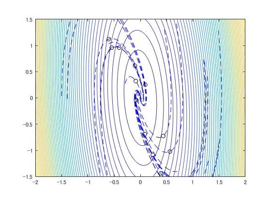
MATLAB Live Script File
A MATLAB live script file is placed at the following link. This is explained in detail in the video on Lyapunov's stability criterion.
Videos Related to Stability
The following is a video explaining poles and stability of systems represented by state equations.
The following is a video explaining Lyapunov's method for systems represented by state equations.
Related Articles